
Sienna Cost Representations
Quick links: reference page on various cost representations, tutorial on operating costs. Substantial implementation pull requests: 1, 2, 3, 4, 5 for part (a) and 6, 7 for part (b). More robust documentation on MarketBidCost hopefully coming soon!
Besides PowerAnalytics.jl, another of my major contributions to the Julia open-source power grid simulation platform Sienna at the National Renewable Energy Lab has been the major upgrade to its cost functions, used in every power generator and storage representation and certain load representations. Before this project, cost functions were stored as raw tuples of numbers, with very little room for the multiple kinds of representations that we wanted to support. My work has had two major phases: (a) the creation of more expressive cost function data structures and (b) the integration of certain features enabled by these data structures into the mathematical optimization problems at the heart of our power grid simulations.
More expressive data structures
A major goal in the design of the cost function data structures was to be able to represent data in whatever form the user might pass in while maintaining an unambiguous physical interpretation of the data. I settled on a multi-tiered design; in order of increasing level of abstraction:
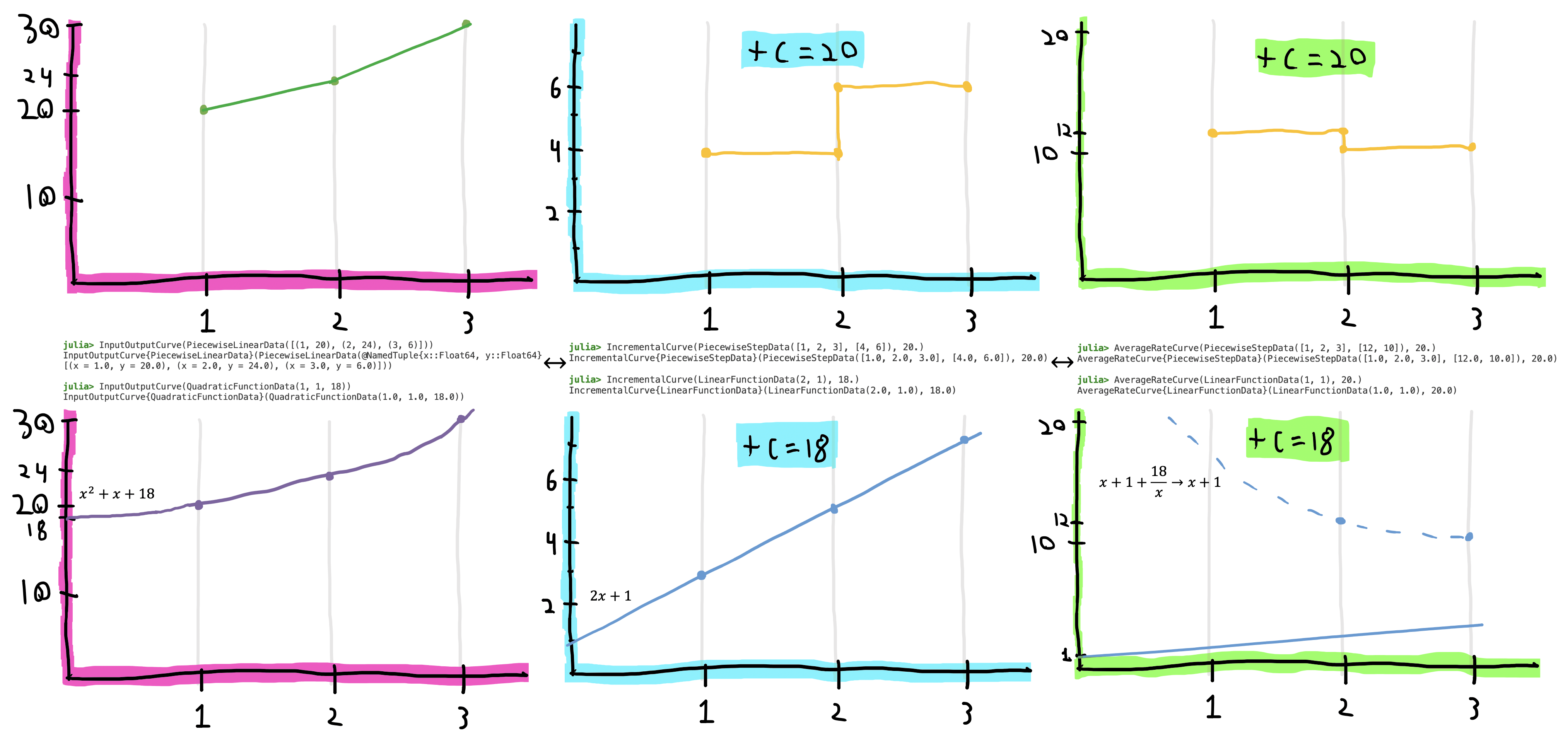
FunctionData: the raw functional representation of the data, able to represent linear, quadratic, piecewise linear, and piecewise stepwise curves.ValueCurve: wraps aFunctionDataand gives it some physical meaning: either anInputOutputCurvethat relates production level (e.g., megawatts) on the x-axis to rate of consumption of inputs (dollars per hour, gallons per hour, etc.) on the y-axis, anIncrementalCurvethat represents marginal costs such that the y-axis is in inputs per additional unit of production, or anAverageCostCurve. These three representations are completely isomorphic: for an input-output curve $y = f(x)$, the incremental curve is the derivative $\frac{dy}{dx}$ and the average cost curve is the expression $\frac{f(x)}{x}$; initial values are automatically stored such that one can convert between the three representations with no data loss up to floating-point precision — see image above.- A
ProductionVariableCostCurve, either aFuelCurveor aCostCurve, specifies either that the y-axis is in terms of currency or that it is in terms of fuel quantity, in which case a fuel cost scalar or time series may be provided. - Various
OperationalCosttypes, such asThermalGenerationCost,StorageCost, andMarketBidCost, combine theProductionVariableCostCurvewith extra domain-specific parameters to fully specify the cost of operating the device at a particular setpoint.
This hierarchy enables a robust, mathematically sound approach to cost functions, but it’s a little unwieldy for users, so various aliases and helpers simplify the interface — see this tutorial for how a user might interact with this design.
More sophisticated simulation
A key feature enabled by this design is the simulation of a power market that takes time-variable piecewise marginal cost bids and dispatches the least-cost configuration of generation to meet demand. I helped solidify the mathematical formulation of a generator driven by such a MarketBidCost, a simplified version of which looks like this:
where $u$, $v$, and $w$ are the on, startup, and shutdown binary variables, $\delta_k$ is the $k$th piecewise tranche variable, $C^{mg}$, $C^{start}$, and $C^{stop}$ are minimum generation, startup, and shutdown costs, $M_k$ is the $k$th piecewise marginal cost, $P^{min}$ and $P^{max}$ are the minimum and maximum generation power, $P_k$ is the $k$th piecewise power breakpoint above the minimum, $t \in \mathcal{T}$ is time, and $P^{min} u_t + \sum_{k \in \mathcal{K}} M_{k, t} \delta_{k, t}$ is the expression for power output to be used elsewhere in the optimization problem.
After a collaborator implemented the non-time-variable version of this formulation, I made it time-variable. To our knowledge, this is the first time this capability has been directly supported in a production cost modeling software suite.